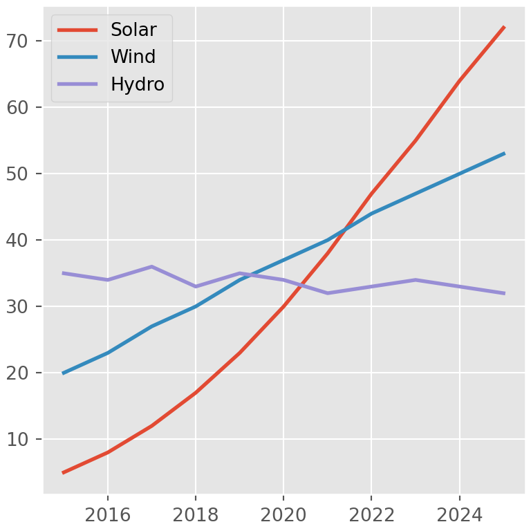
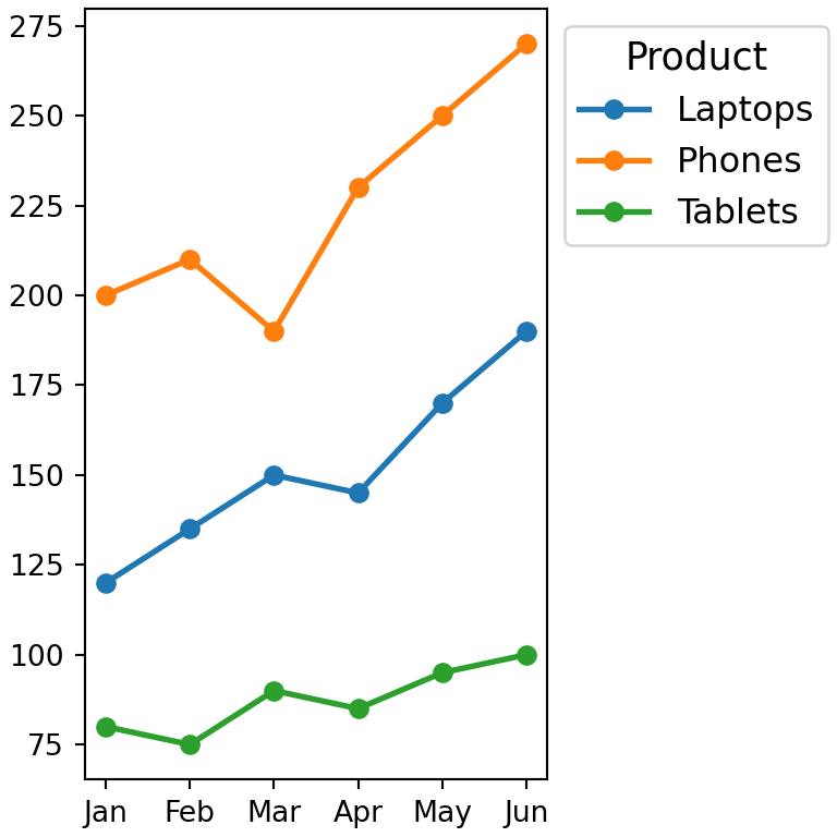
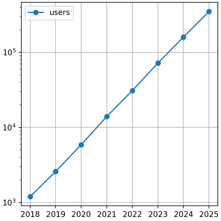
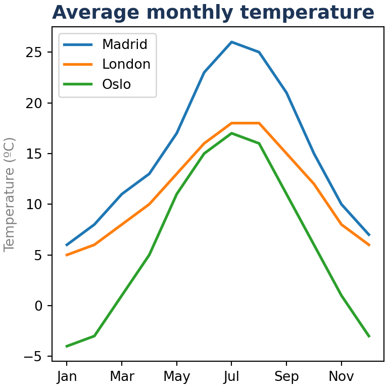
pandas DataFrames and Series have a plot method that creates charts with matplotlib in a single line of code. The index is used for the X axis and each column becomes a series, so it is the fastest way to explore your data visually.
The plot method
By default plot creates a line chart with one line for each numeric column of the data frame.
import numpy as np
import pandas as pd
import matplotlib.pyplot as plt

rng = np.random.default_rng(1)
df = pd.DataFrame(rng.normal(size = (100, 3)).cumsum(axis = 0),
                  columns = ["A", "B", "C"],
                  index = pd.date_range("2025-01-01", periods = 100))

df.plot()
# plt.show()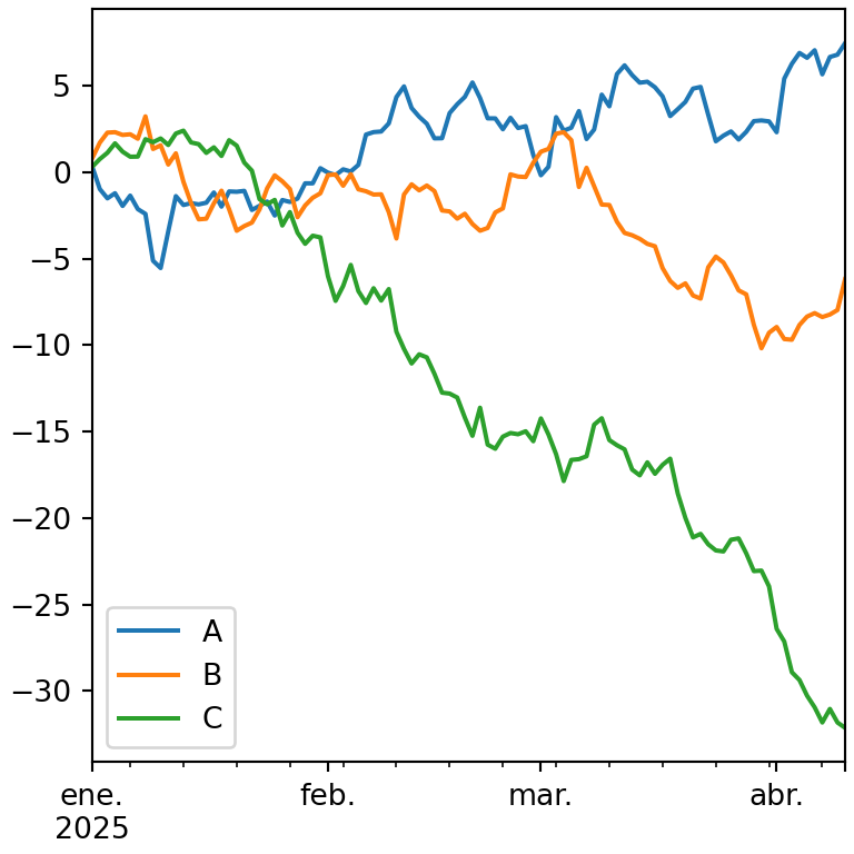
Select the columns
Use x and y to choose the columns. y also accepts a list of columns.
import pandas as pd
import matplotlib.pyplot as plt

df = pd.DataFrame({"month": ["Jan", "Feb", "Mar", "Apr", "May", "Jun"],
                   "sales": [12, 15, 14, 18, 21, 19],
                   "costs": [8, 9, 9, 11, 12, 12]})

df.plot(x = "month", y = ["sales", "costs"])
# plt.show()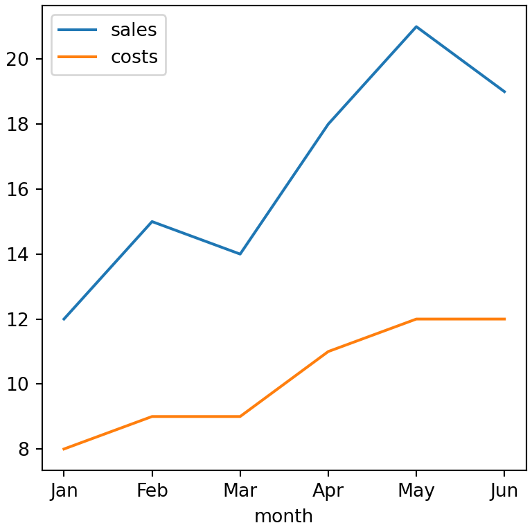
Types of charts with kind
The kind argument sets the type of chart. Each type also has its own method in the plot accessor, so df.plot(kind = "bar") is the same as df.plot.bar().
| kind | Method | Chart |
|---|---|---|
“line”
|
plot.line()
|
Line chart |
“bar” / “barh”
|
plot.bar() / plot.barh()
|
Bar chart |
“hist”
|
plot.hist()
|
Histogram |
“box”
|
plot.box()
|
Box plot |
“kde” / “density”
|
plot.kde()
|
Density plot |
“area”
|
plot.area()
|
Area chart |
“pie”
|
plot.pie()
|
Pie chart |
“scatter”
|
plot.scatter()
|
Scatter plot |
“hexbin”
|
plot.hexbin()
|
Hexbin chart |
import pandas as pd
import matplotlib.pyplot as plt

df = pd.DataFrame({"sales": [12, 18, 9, 15],
                   "costs": [8, 11, 7, 10]},
                  index = ["Q1", "Q2", "Q3", "Q4"])

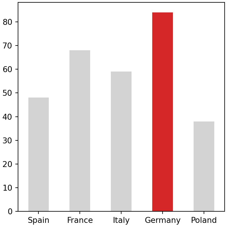
df.plot(kind = "bar")
# plt.show()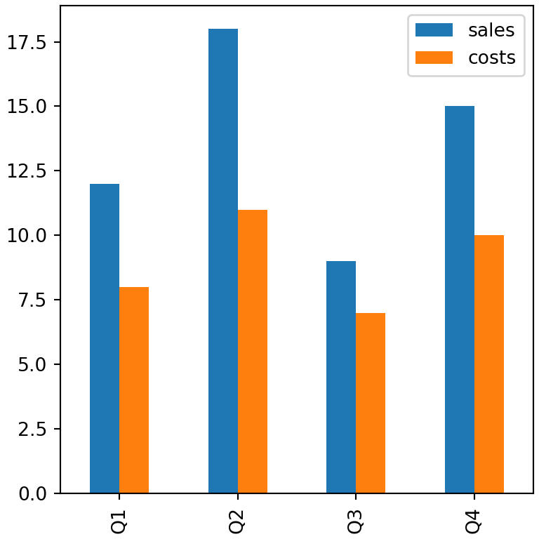
Customizing the chart
plot accepts many arguments to customize the chart: title, xlabel, ylabel, figsize, color, grid, legend, rot (rotation of the tick labels), xlim, ylim, logy and others.
import pandas as pd
import matplotlib.pyplot as plt

df = pd.DataFrame({"sales": [12, 18, 9, 15],
                   "costs": [8, 11, 7, 10]},
                  index = ["Q1", "Q2", "Q3", "Q4"])

df.plot(kind = "bar", title = "Quarterly results",
        xlabel = "Quarter", ylabel = "Euros",
        color = ["#2A9D8F", "#E76F51"], rot = 0, grid = True)
# plt.show()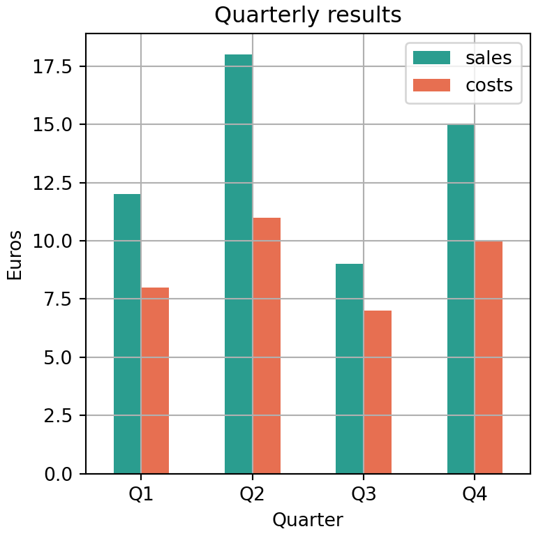
Colormap
Instead of listing the colors you can pass a matplotlib colormap with colormap.
import numpy as np
import pandas as pd
import matplotlib.pyplot as plt

rng = np.random.default_rng(1)
df = pd.DataFrame(rng.normal(size = (100, 3)).cumsum(axis = 0),
                  columns = ["A", "B", "C"],
                  index = pd.date_range("2025-01-01", periods = 100))

df.plot(colormap = "viridis")
# plt.show()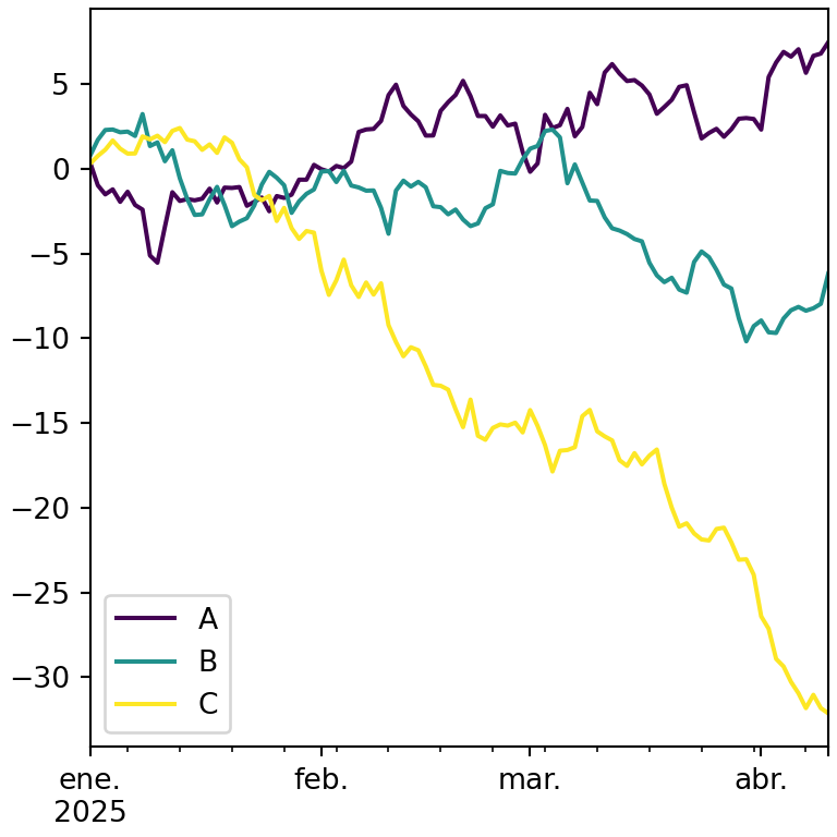
Line styles
The style argument accepts a matplotlib format string for each column.
import numpy as np
import pandas as pd
import matplotlib.pyplot as plt

rng = np.random.default_rng(1)
df = pd.DataFrame(rng.normal(size = (100, 3)).cumsum(axis = 0),
                  columns = ["A", "B", "C"],
                  index = pd.date_range("2025-01-01", periods = 100))

df.plot(style = ["-", "--", ":"])
# plt.show()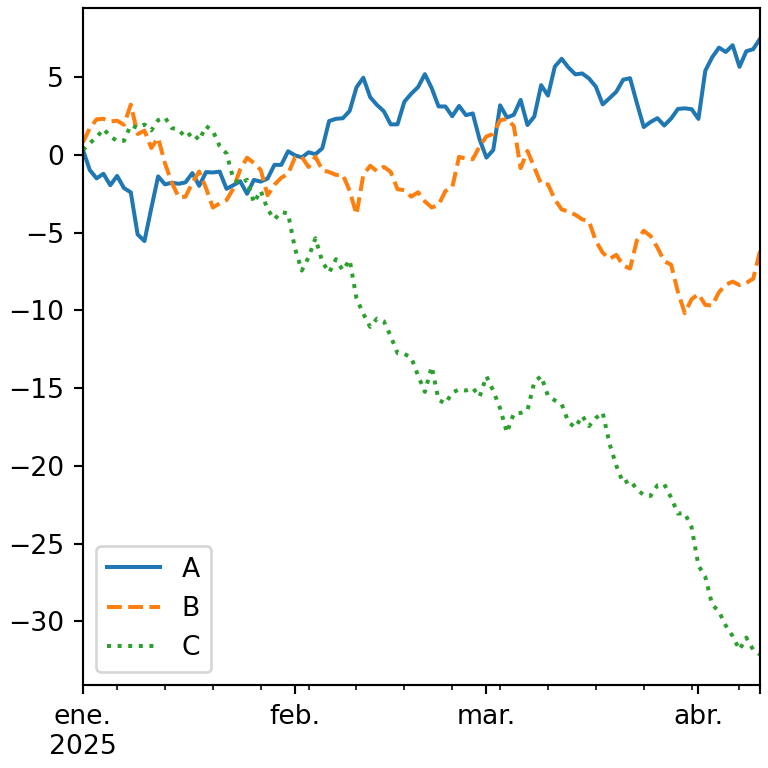
One subplot per column
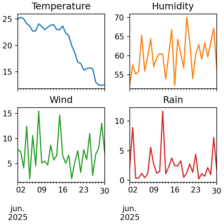
Set subplots = True to draw each column in its own subplot. Use layout to choose the number of rows and columns and sharey to share the Y axis.
import numpy as np
import pandas as pd
import matplotlib.pyplot as plt

rng = np.random.default_rng(1)
df = pd.DataFrame(rng.normal(size = (100, 3)).cumsum(axis = 0),
                  columns = ["A", "B", "C"],
                  index = pd.date_range("2025-01-01", periods = 100))

df.plot(subplots = True, layout = (3, 1), sharex = True)
# plt.show()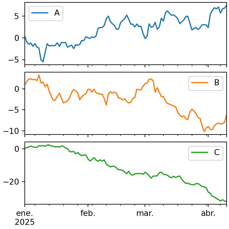
Secondary Y axis
When the columns have different scales, pass the name of one or several columns to secondary_y to draw them on a second axis.
import pandas as pd
import matplotlib.pyplot as plt

df = pd.DataFrame({"sales": [120, 150, 140, 180, 210, 190],
                   "margin": [0.12, 0.15, 0.13, 0.18, 0.2, 0.17]})

df.plot(secondary_y = "margin")
# plt.show()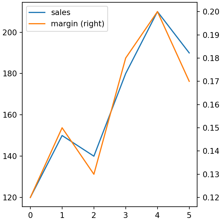
Further customization with matplotlib
plot returns a matplotlib axes object, so you can keep customizing the chart with all the matplotlib methods, for instance adding a reference line or formatting the axis.
import pandas as pd
import matplotlib.pyplot as plt

df = pd.DataFrame({"sales": [12, 18, 9, 15],
                   "costs": [8, 11, 7, 10]},
                  index = ["Q1", "Q2", "Q3", "Q4"])

ax = df.plot(kind = "bar", rot = 0)

ax.axhline(14, color = "black", linestyle = "--", label = "Target")
ax.spines[["top", "right"]].set_visible(False)
ax.legend()
# plt.show()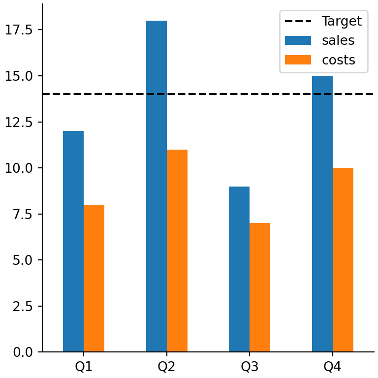
Interactive charts with plotly as backend
pandas can also use other plotting libraries. If you have plotly installed, change the backend to create interactive charts with the same syntax:
import pandas as pd

pd.options.plotting.backend = "plotly"

df = pd.DataFrame({"sales": [12, 18, 9, 15], "costs": [8, 11, 7, 10]})
fig = df.plot(kind = "bar")
fig.show()
Learn more about each type of chart in the line chart, bar chart, histogram, box plot, scatter plot, area chart and pie chart tutorials. To customize the charts see the guides about titles, axes, legend, colors, subplots and size and styles.