Dendrogram in Python with scipy and matplotlib

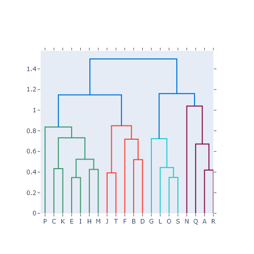
A dendrogram is a tree diagram that shows the result of a hierarchical clustering: the observations that are joined lower in the tree are more similar. In Python the clustering is computed with linkage from scipy.cluster.hierarchy and the tree is drawn with dendrogram. The examples use data about car crashes in 20 US states.

Dendrogram with linkage and dendrogram

linkage computes the hierarchical clustering (here with the Ward method) and dendrogram draws it on the current matplotlib axes.

import seaborn as sns
import matplotlib.pyplot as plt
from scipy.cluster.hierarchy import linkage, dendrogram

crashes = sns.load_dataset("car_crashes").set_index("abbrev").head(20)
Z = linkage(crashes[["speeding", "alcohol", "not_distracted", "no_previous"]], method = "ward")

fig, ax = plt.subplots()
dendrogram(Z, labels = crashes.index.tolist(), ax = ax)
# plt.show()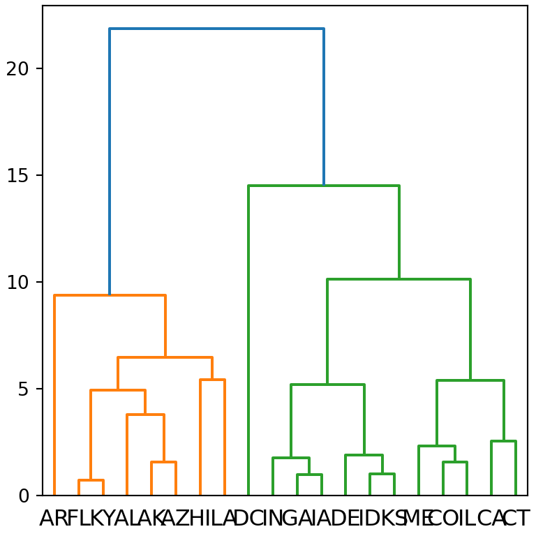

Horizontal dendrogram

orientation places the root of the tree on the "top" (default), "bottom", "left" or "right". A horizontal dendrogram leaves more space for the labels.

import seaborn as sns
import matplotlib.pyplot as plt
from scipy.cluster.hierarchy import linkage, dendrogram

crashes = sns.load_dataset("car_crashes").set_index("abbrev").head(20)
Z = linkage(crashes[["speeding", "alcohol", "not_distracted", "no_previous"]], method = "ward")

fig, ax = plt.subplots()
dendrogram(Z, labels = crashes.index.tolist(), orientation = "left", ax = ax)
# plt.show()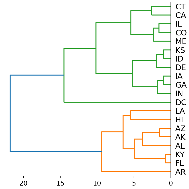

Color the clusters with a threshold

color_threshold sets the height at which the tree is cut: each cluster below that height gets a different color. Draw the cut with axhline to make it visible.

import seaborn as sns
import matplotlib.pyplot as plt
from scipy.cluster.hierarchy import linkage, dendrogram

crashes = sns.load_dataset("car_crashes").set_index("abbrev").head(20)
Z = linkage(crashes[["speeding", "alcohol", "not_distracted", "no_previous"]], method = "ward")

fig, ax = plt.subplots()
dendrogram(Z, labels = crashes.index.tolist(), color_threshold = 15,
           above_threshold_color = "gray", ax = ax)
ax.axhline(15, color = "black", linestyle = "--")
# plt.show()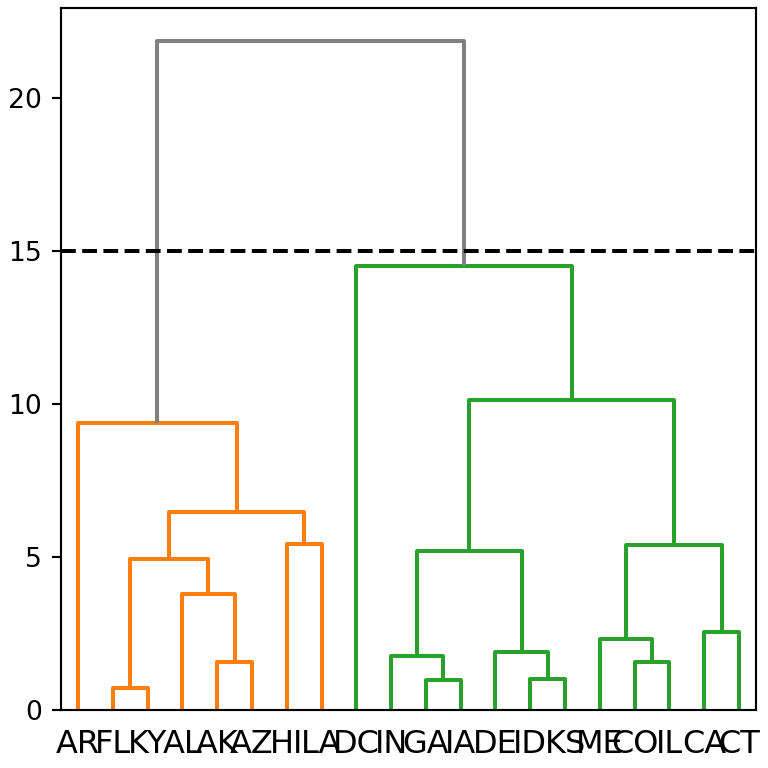

Truncate the dendrogram

With many observations the tree is hard to read. truncate_mode = "lastp" shows only the last p merged clusters; the number of observations of each one is displayed between parentheses.

import seaborn as sns
import matplotlib.pyplot as plt
from scipy.cluster.hierarchy import linkage, dendrogram

crashes = sns.load_dataset("car_crashes").set_index("abbrev")
Z = linkage(crashes[["speeding", "alcohol", "not_distracted", "no_previous"]], method = "ward")

fig, ax = plt.subplots()
dendrogram(Z, truncate_mode = "lastp", p = 8, ax = ax)
# plt.show()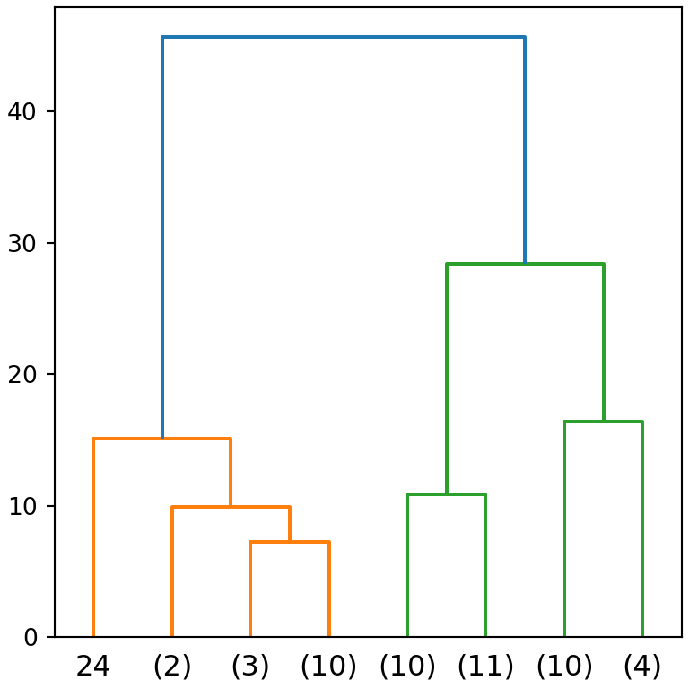

Linkage methods

The shape of the tree depends on the method used to measure the distance between clusters: "ward", "complete", "average", "single"…

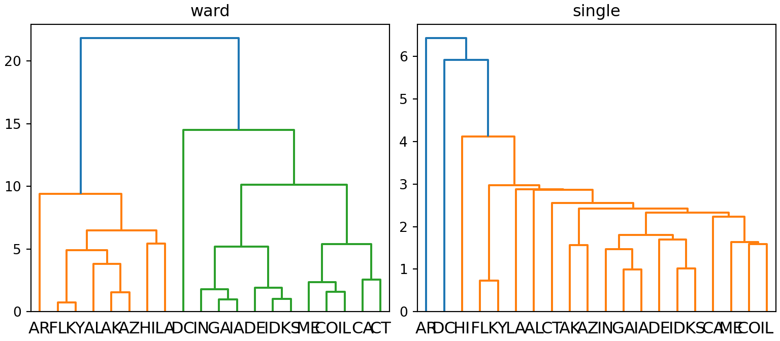
import seaborn as sns
import matplotlib.pyplot as plt
from scipy.cluster.hierarchy import linkage, dendrogram

crashes = sns.load_dataset("car_crashes").set_index("abbrev").head(20)
X = crashes[["speeding", "alcohol", "not_distracted", "no_previous"]]

fig, axs = plt.subplots(1, 2, figsize = (8, 3.5))
for ax, method in zip(axs, ["ward", "single"]):
    dendrogram(linkage(X, method = method), labels = X.index.tolist(), ax = ax)
    ax.set_title(method)
# plt.show()

To combine the dendrogram with a heat map use the clustermap of seaborn. See also the dendrogram in plotly.