A connection map shows the links between places, such as flight routes, trade or migrations. The base map is drawn with geopandas and the connections are lines between the coordinates of the places. The examples show some flight routes from Madrid.
Routes as straight lines
Draw the world map and add a line from the origin to each destination with plot, using the longitude as X and the latitude as Y.
import numpy as np
import geopandas as gpd
import matplotlib.pyplot as plt

world = gpd.read_file("https://naciscdn.org/naturalearth/110m/cultural/ne_110m_admin_0_countries.zip")
cities = {"Madrid": (-3.7, 40.4), "New York": (-74.0, 40.7), "Sao Paulo": (-46.6, -23.5),
          "Tokyo": (139.7, 35.7), "Sydney": (151.2, -33.9), "Johannesburg": (28.0, -26.2),
          "Moscow": (37.6, 55.8), "Mexico City": (-99.1, 19.4)}

fig, ax = plt.subplots()
world.plot(ax = ax, color = "lightgray", edgecolor = "white", linewidth = 0.3)

origin = cities["Madrid"]
for name, dest in cities.items():
    ax.plot([origin[0], dest[0]], [origin[1], dest[1]], color = "tab:red")
ax.axis("off")
# plt.show()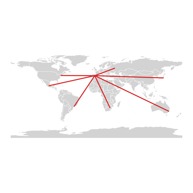
Great circle arcs
The shortest route between two points of the Earth is an arc of a great circle, not a straight line on the map. The following function computes the points of that arc, so the routes look like real flight paths.
import numpy as np
import geopandas as gpd
import matplotlib.pyplot as plt

world = gpd.read_file("https://naciscdn.org/naturalearth/110m/cultural/ne_110m_admin_0_countries.zip")
cities = {"Madrid": (-3.7, 40.4), "New York": (-74.0, 40.7), "Sao Paulo": (-46.6, -23.5),
          "Tokyo": (139.7, 35.7), "Sydney": (151.2, -33.9), "Johannesburg": (28.0, -26.2),
          "Moscow": (37.6, 55.8), "Mexico City": (-99.1, 19.4)}

def great_circle(p1, p2, n = 100):
    """Points of the great circle between two (lon, lat) points."""
    lon1, lat1, lon2, lat2 = np.radians([*p1, *p2])
    a = np.array([np.cos(lat1) * np.cos(lon1), np.cos(lat1) * np.sin(lon1), np.sin(lat1)])
    b = np.array([np.cos(lat2) * np.cos(lon2), np.cos(lat2) * np.sin(lon2), np.sin(lat2)])
    omega = np.arccos(np.clip(a @ b, -1, 1))
    t = np.linspace(0, 1, n)[:, None]
    p = (np.sin((1 - t) * omega) * a + np.sin(t * omega) * b) / np.sin(omega)
    return np.degrees(np.arctan2(p[:, 1], p[:, 0])), np.degrees(np.arcsin(p[:, 2]))

fig, ax = plt.subplots()
world.plot(ax = ax, color = "lightgray", edgecolor = "white", linewidth = 0.3)

for name, dest in cities.items():
    if name != "Madrid":
        lon, lat = great_circle(cities["Madrid"], dest)
        ax.plot(lon, lat, color = "tab:red")
ax.axis("off")
# plt.show()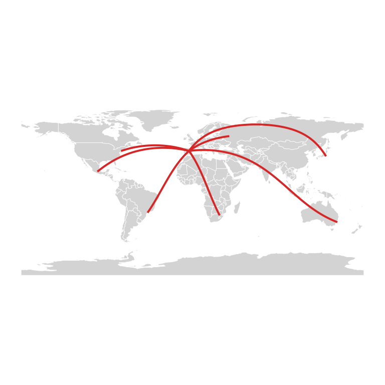
Width by a variable
Set the width of each route according to a variable, for example the number of weekly flights, and mark the cities with points.
import numpy as np
import geopandas as gpd
import matplotlib.pyplot as plt

world = gpd.read_file("https://naciscdn.org/naturalearth/110m/cultural/ne_110m_admin_0_countries.zip")
cities = {"Madrid": (-3.7, 40.4), "New York": (-74.0, 40.7), "Sao Paulo": (-46.6, -23.5),
          "Tokyo": (139.7, 35.7), "Sydney": (151.2, -33.9), "Johannesburg": (28.0, -26.2),
          "Moscow": (37.6, 55.8), "Mexico City": (-99.1, 19.4)}

def great_circle(p1, p2, n = 100):
    """Points of the great circle between two (lon, lat) points."""
    lon1, lat1, lon2, lat2 = np.radians([*p1, *p2])
    a = np.array([np.cos(lat1) * np.cos(lon1), np.cos(lat1) * np.sin(lon1), np.sin(lat1)])
    b = np.array([np.cos(lat2) * np.cos(lon2), np.cos(lat2) * np.sin(lon2), np.sin(lat2)])
    omega = np.arccos(np.clip(a @ b, -1, 1))
    t = np.linspace(0, 1, n)[:, None]
    p = (np.sin((1 - t) * omega) * a + np.sin(t * omega) * b) / np.sin(omega)
    return np.degrees(np.arctan2(p[:, 1], p[:, 0])), np.degrees(np.arcsin(p[:, 2]))

flights = {"New York": 28, "Sao Paulo": 14, "Tokyo": 7, "Sydney": 3,
           "Johannesburg": 5, "Moscow": 10, "Mexico City": 21}

fig, ax = plt.subplots()
world.plot(ax = ax, color = "lightgray", edgecolor = "white", linewidth = 0.3)

for name, n in flights.items():
    lon, lat = great_circle(cities["Madrid"], cities[name])
    ax.plot(lon, lat, color = "tab:red", linewidth = n / 5, alpha = 0.7)
xy = np.array(list(cities.values()))
ax.scatter(xy[:, 0], xy[:, 1], s = 15, color = "black", zorder = 3)
ax.axis("off")
# plt.show()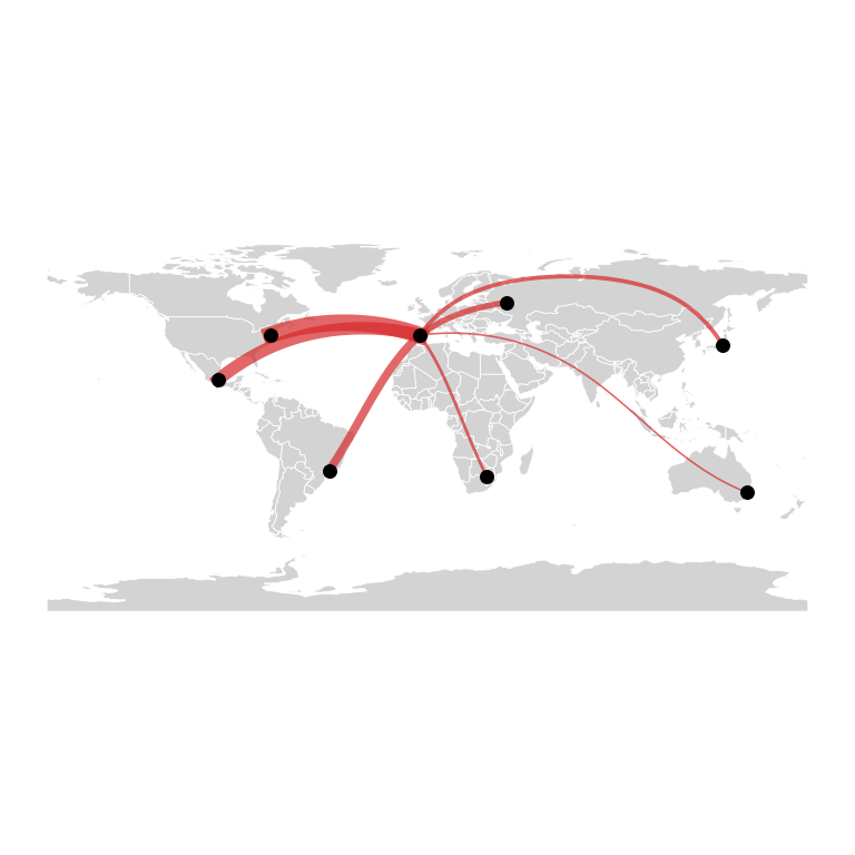
Map style
A dark background with bright routes is a classic look for this kind of map. Add the names of the cities with text.
import numpy as np
import geopandas as gpd
import matplotlib.pyplot as plt

world = gpd.read_file("https://naciscdn.org/naturalearth/110m/cultural/ne_110m_admin_0_countries.zip")
cities = {"Madrid": (-3.7, 40.4), "New York": (-74.0, 40.7), "Sao Paulo": (-46.6, -23.5),
          "Tokyo": (139.7, 35.7), "Sydney": (151.2, -33.9), "Johannesburg": (28.0, -26.2),
          "Moscow": (37.6, 55.8), "Mexico City": (-99.1, 19.4)}

def great_circle(p1, p2, n = 100):
    """Points of the great circle between two (lon, lat) points."""
    lon1, lat1, lon2, lat2 = np.radians([*p1, *p2])
    a = np.array([np.cos(lat1) * np.cos(lon1), np.cos(lat1) * np.sin(lon1), np.sin(lat1)])
    b = np.array([np.cos(lat2) * np.cos(lon2), np.cos(lat2) * np.sin(lon2), np.sin(lat2)])
    omega = np.arccos(np.clip(a @ b, -1, 1))
    t = np.linspace(0, 1, n)[:, None]
    p = (np.sin((1 - t) * omega) * a + np.sin(t * omega) * b) / np.sin(omega)
    return np.degrees(np.arctan2(p[:, 1], p[:, 0])), np.degrees(np.arcsin(p[:, 2]))

fig, ax = plt.subplots(facecolor = "#0B1D33")
world.plot(ax = ax, color = "#1F3A5F", edgecolor = "#0B1D33", linewidth = 0.3)

for name, dest in cities.items():
    if name != "Madrid":
        lon, lat = great_circle(cities["Madrid"], dest)
        ax.plot(lon, lat, color = "#FFD166", linewidth = 4, alpha = 0.15)
        ax.plot(lon, lat, color = "#FFD166", linewidth = 1)
for name, (x, y) in cities.items():
    ax.scatter(x, y, color = "white", s = 10, zorder = 3)
    ax.text(x, y - 7, name, color = "white", fontsize = 6, ha = "center")
ax.set_ylim(-60, 85)
ax.axis("off")
# plt.show()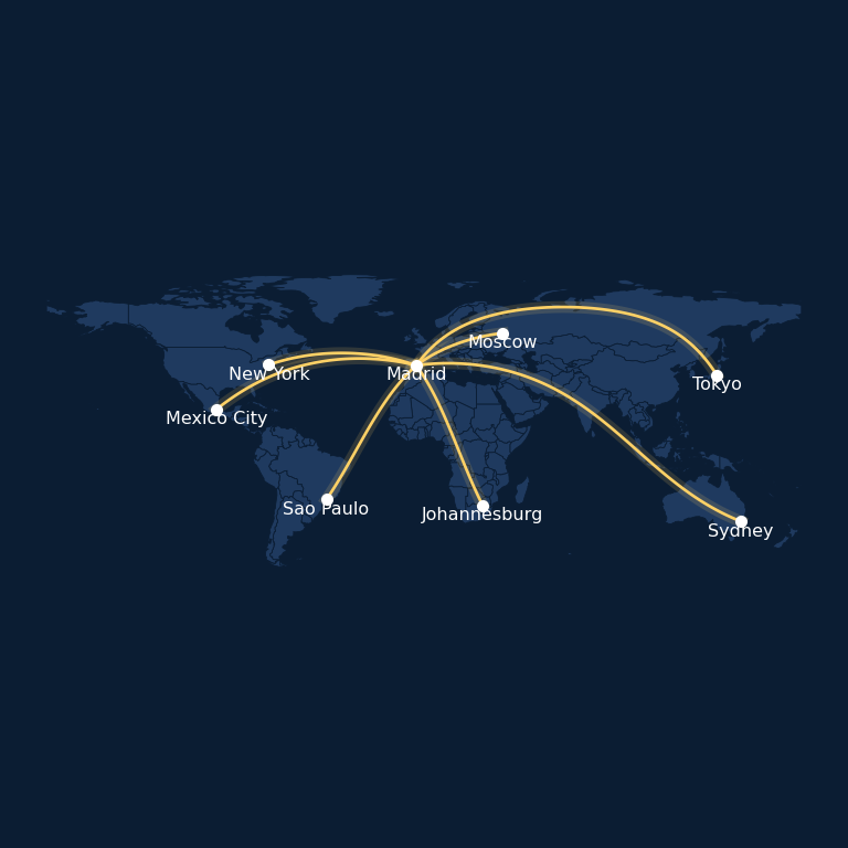
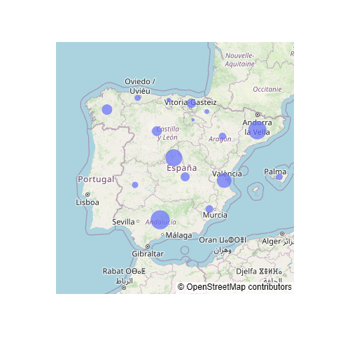
See also how to create a static map with geopandas and an interactive bubble map in plotly.