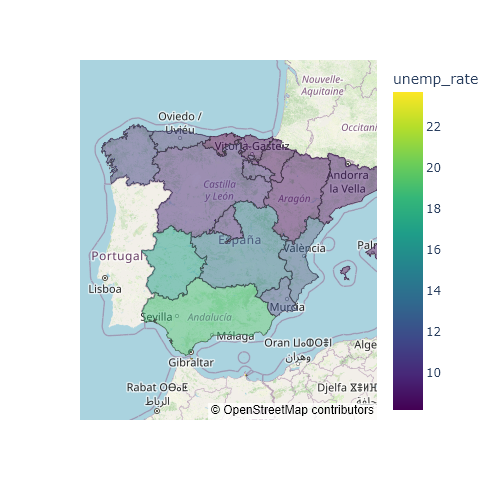
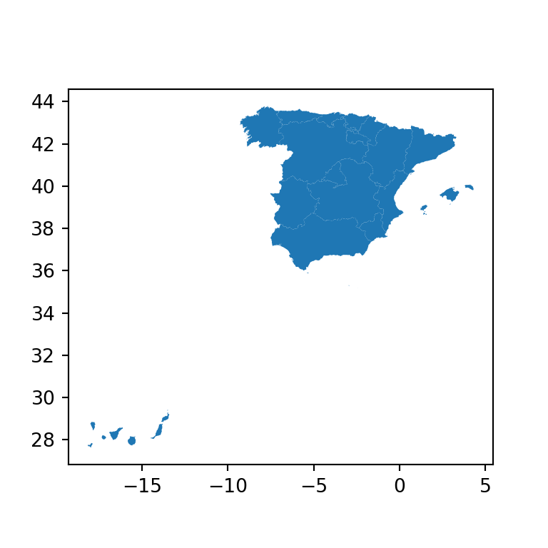
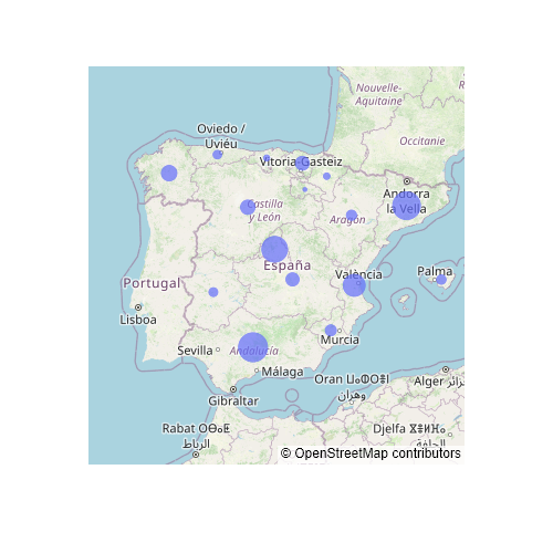
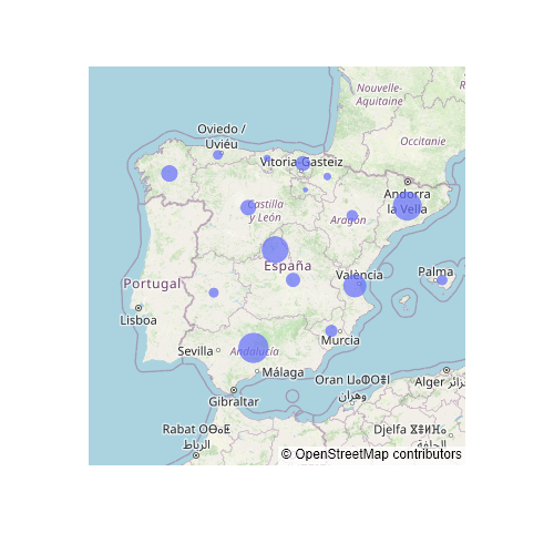
A choropleth map colors each region according to the value of a variable. With geopandas you can read a shapefile or a GeoJSON file into a GeoDataFrame and draw it with its plot method, which uses matplotlib. The examples show the unemployment rate (%) of the autonomous communities of Spain; the Canary Islands are moved closer to the peninsula with translate, as is usual in maps of Spain.
Choropleth map with plot
Pass the name of the column to represent to the column argument of plot. legend = True adds a color bar.
import geopandas as gpd
import matplotlib.pyplot as plt

spain = gpd.read_file("https://raw.githubusercontent.com/R-CoderDotCom/data/main/shapefile_spain/spain.zip")

# Move the Canary Islands closer to the peninsula
canarias = spain["name"] == "Islas Canarias"
spain.loc[canarias, "geometry"] = spain[canarias].translate(xoff = 5, yoff = 6.5)

fig, ax = plt.subplots()
spain.plot(column = "unemp_rate", legend = True, ax = ax)
ax.axis("off")
# plt.show()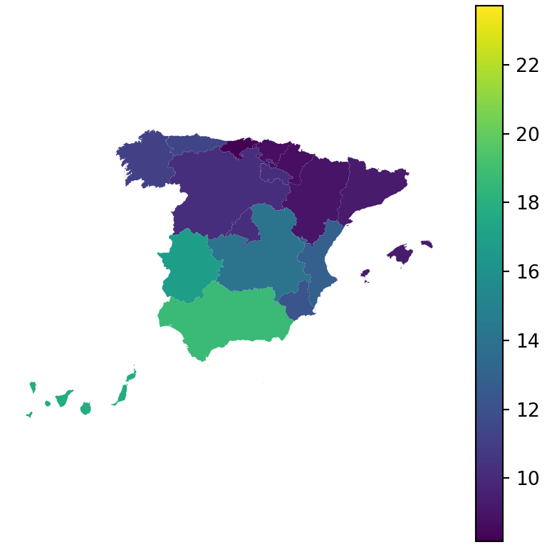
Colormap and borders
Choose the colors with cmap and customize the borders of the regions with edgecolor and linewidth.
import geopandas as gpd
import matplotlib.pyplot as plt

spain = gpd.read_file("https://raw.githubusercontent.com/R-CoderDotCom/data/main/shapefile_spain/spain.zip")

# Move the Canary Islands closer to the peninsula
canarias = spain["name"] == "Islas Canarias"
spain.loc[canarias, "geometry"] = spain[canarias].translate(xoff = 5, yoff = 6.5)

fig, ax = plt.subplots()
spain.plot(column = "unemp_rate", cmap = "Reds",
           edgecolor = "white", linewidth = 0.8, legend = True, ax = ax)
ax.axis("off")
# plt.show()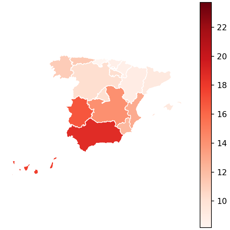
Legend customization
legend_kwds passes arguments to the color bar, such as its label, its orientation or its size with shrink.
import geopandas as gpd
import matplotlib.pyplot as plt

spain = gpd.read_file("https://raw.githubusercontent.com/R-CoderDotCom/data/main/shapefile_spain/spain.zip")

# Move the Canary Islands closer to the peninsula
canarias = spain["name"] == "Islas Canarias"
spain.loc[canarias, "geometry"] = spain[canarias].translate(xoff = 5, yoff = 6.5)

fig, ax = plt.subplots()
spain.plot(column = "unemp_rate", cmap = "YlOrRd", edgecolor = "white", linewidth = 0.6,
           legend = True, ax = ax,
           legend_kwds = {"label": "Unemployment rate (%)",
                          "orientation": "horizontal", "shrink": 0.7})
ax.set_title("Unemployment in Spain", fontsize = 14)
ax.axis("off")
# plt.show()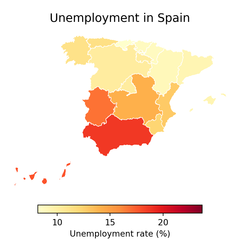
Group the values in classes
Instead of a continuous scale you can group the values in intervals with pd.cut and represent them as a categorical variable with categorical = True.
import geopandas as gpd
import matplotlib.pyplot as plt

spain = gpd.read_file("https://raw.githubusercontent.com/R-CoderDotCom/data/main/shapefile_spain/spain.zip")

# Move the Canary Islands closer to the peninsula
canarias = spain["name"] == "Islas Canarias"
spain.loc[canarias, "geometry"] = spain[canarias].translate(xoff = 5, yoff = 6.5)
import pandas as pd

spain["level"] = pd.cut(spain["unemp_rate"], bins = [0, 10, 15, 30],
                        labels = ["Low", "Medium", "High"])

fig, ax = plt.subplots()
spain.plot(column = "level", categorical = True, cmap = "RdYlGn_r",
           legend = True, edgecolor = "white", ax = ax)
ax.axis("off")
# plt.show()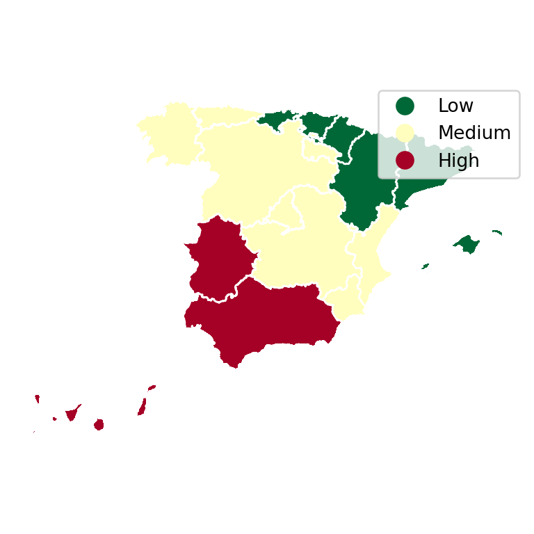
Labels on the regions
Write the value of each region at a point inside it, obtained with representative_point.
import geopandas as gpd
import matplotlib.pyplot as plt

spain = gpd.read_file("https://raw.githubusercontent.com/R-CoderDotCom/data/main/shapefile_spain/spain.zip")

# Move the Canary Islands closer to the peninsula
canarias = spain["name"] == "Islas Canarias"
spain.loc[canarias, "geometry"] = spain[canarias].translate(xoff = 5, yoff = 6.5)

fig, ax = plt.subplots()
spain.plot(column = "unemp_rate", cmap = "Blues", edgecolor = "white", ax = ax)

for geom, value in zip(spain.geometry, spain["unemp_rate"]):
    p = geom.representative_point()
    ax.annotate(f"{value:.0f}", (p.x, p.y), ha = "center", fontsize = 7)
ax.axis("off")
# plt.show()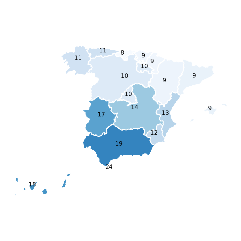
To create an interactive choropleth map see the choropleth map in plotly tutorial, and for the basics of geopandas the static maps with geopandas tutorial.