Seaborn adds a legend automatically when you map a variable to hue, style or size. The legend can be customized with the sns.move_legend function, available since seaborn 0.11.2, and with the legend methods of matplotlib.
Default legend
Grouping the data with hue creates a legend with one entry per group. The title of the legend is the name of the column.
import seaborn as sns
import matplotlib.pyplot as plt

mpg = sns.load_dataset("mpg")

sns.scatterplot(data = mpg, x = "horsepower", y = "mpg", hue = "origin")
# plt.show()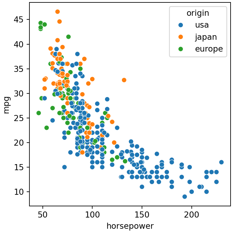
Legend position with move_legend
sns.move_legend changes the position of an existing legend. Its first argument is the axes (or the object returned by a figure-level function) and the second the location, with the same values as in matplotlib: "upper left", "lower right", "center"…
import seaborn as sns
import matplotlib.pyplot as plt

mpg = sns.load_dataset("mpg")

ax = sns.scatterplot(data = mpg, x = "horsepower", y = "mpg", hue = "origin")
sns.move_legend(ax, "lower left")
# plt.show()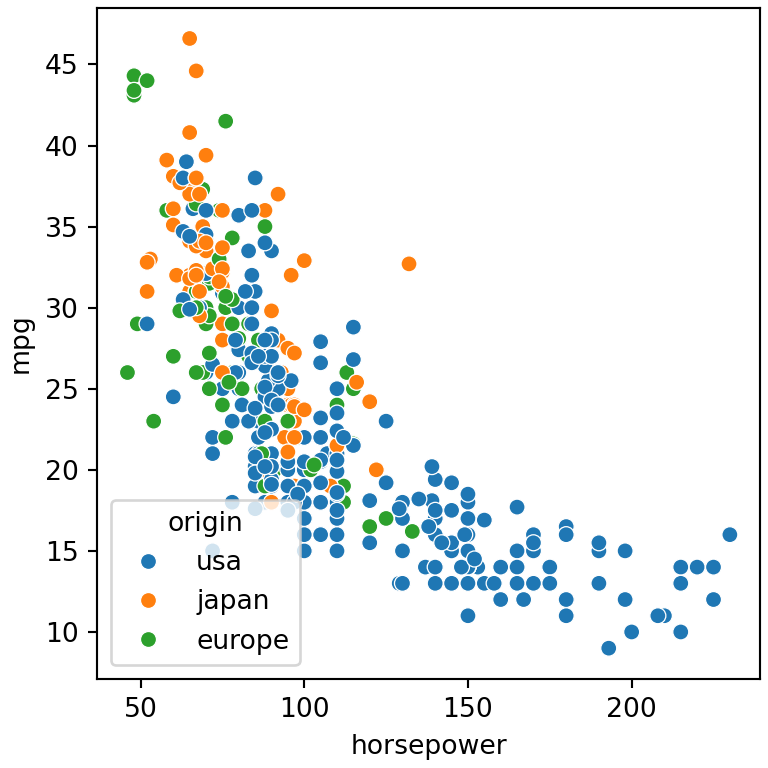
Legend outside the plot
Use bbox_to_anchor to place the legend outside the plot. The following example places the upper left corner of the legend next to the upper right corner of the axes.
import seaborn as sns
import matplotlib.pyplot as plt

mpg = sns.load_dataset("mpg")

ax = sns.scatterplot(data = mpg, x = "horsepower", y = "mpg", hue = "origin", s = 50)
sns.move_legend(ax, "upper left", bbox_to_anchor = (1, 1),
                title = "Origin", fontsize = 12, title_fontsize = 13)
# plt.show()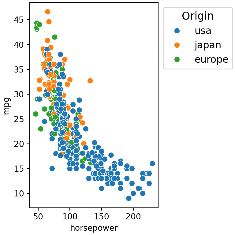
Legend below the plot
For a horizontal legend below the plot set ncol to the number of groups and remove the frame with frameon = False.
import seaborn as sns
import matplotlib.pyplot as plt

mpg = sns.load_dataset("mpg")

ax = sns.scatterplot(data = mpg, x = "horsepower", y = "mpg", hue = "origin")
sns.move_legend(ax, "upper center", bbox_to_anchor = (0.5, -0.15),
                ncol = 3, title = None, frameon = False)
# plt.show()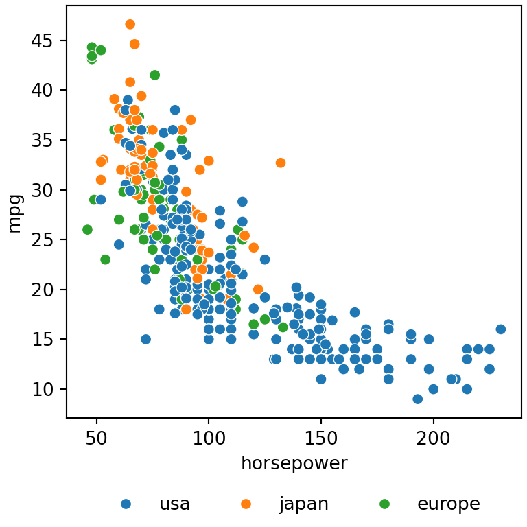
Legend title and labels
move_legend also accepts any argument of the matplotlib legend function, such as title, fontsize or title_fontsize.
import seaborn as sns
import matplotlib.pyplot as plt

mpg = sns.load_dataset("mpg")

ax = sns.scatterplot(data = mpg, x = "horsepower", y = "mpg", hue = "origin")
sns.move_legend(ax, "upper right", title = "Origin",
                fontsize = 9, title_fontsize = 11)
# plt.show()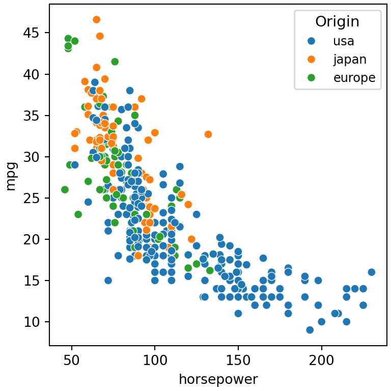
Change the labels
The labels of the legend are the values of the grouping column. The easiest way to change them is renaming the values of the data before plotting it, for instance with replace.
import seaborn as sns
import matplotlib.pyplot as plt

mpg = sns.load_dataset("mpg")

mpg["origin"] = mpg["origin"].replace({"usa": "USA", "europe": "Europe", "japan": "Japan"})

sns.scatterplot(data = mpg, x = "horsepower", y = "mpg", hue = "origin")
# plt.show()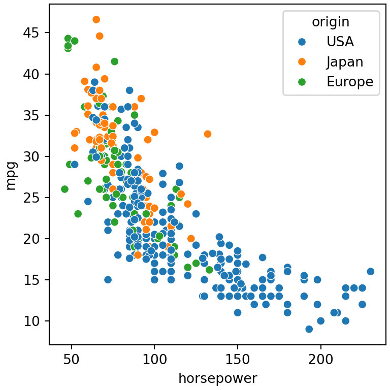
Legend of figure-level functions
Figure-level functions (relplot, displot, catplot…) place the legend outside the plot by default. Pass the returned object to move_legend to change it, or set legend_out = False through facet_kws to draw it inside the plot.
import seaborn as sns
import matplotlib.pyplot as plt

mpg = sns.load_dataset("mpg")

g = sns.displot(data = mpg, x = "mpg", hue = "origin",
                kind = "kde", fill = True, height = 4)
sns.move_legend(g, "upper right", bbox_to_anchor = (0.95, 0.95))
# plt.show()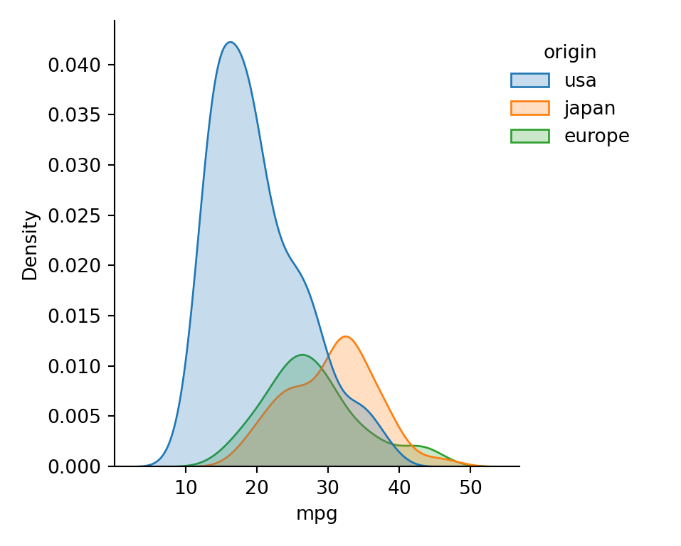
Legend for numeric variables
When hue or size is a numeric variable seaborn shows only some representative values (legend = "brief"). Use legend = "full" to display all the values.
import seaborn as sns
import matplotlib.pyplot as plt

mpg = sns.load_dataset("mpg")

sns.scatterplot(data = mpg, x = "horsepower", y = "mpg",
                hue = "cylinders", size = "cylinders", legend = "full")
# plt.show()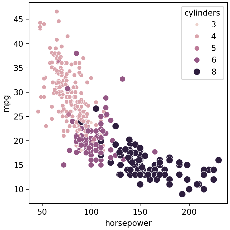
Remove the legend
Set legend = False in the seaborn function to create the plot without legend. If the plot is already created remove it with ax.get_legend().remove().
import seaborn as sns
import matplotlib.pyplot as plt

mpg = sns.load_dataset("mpg")

sns.scatterplot(data = mpg, x = "horsepower", y = "mpg", hue = "origin",
                legend = False)
# plt.show()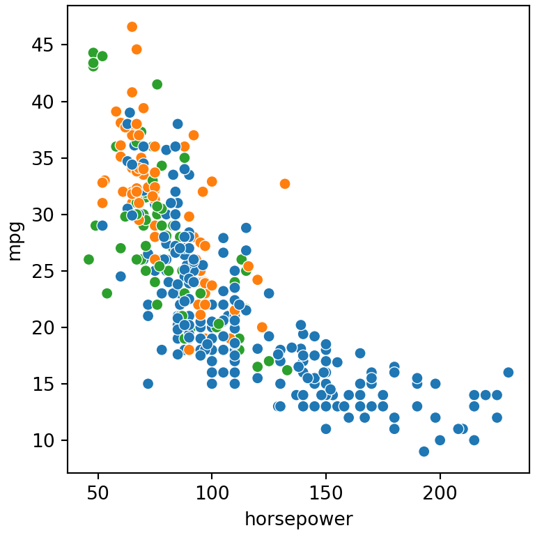
As seaborn is built on top of matplotlib you can also use all the options of the legend in matplotlib. See also how to customize the axes and the titles of seaborn plots.