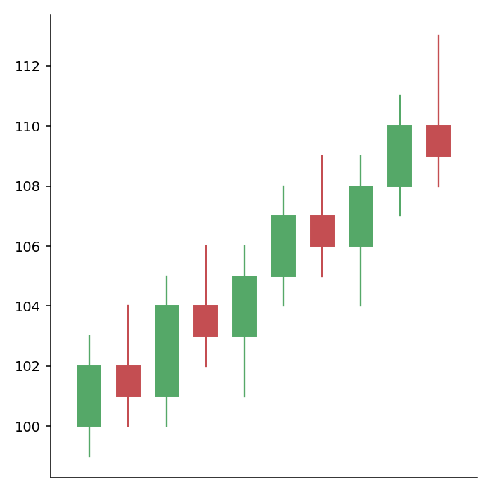
Candlestick charts represent the evolution of the price of an asset: each candle shows the opening, the highest, the lowest and the closing price of a period. The mplfinance library, built on matplotlib, creates them from a pandas data frame with a date index and the columns Open, High, Low, Close and, optionally, Volume.
Candlestick chart with mpf.plot
Pass the data frame to mpf.plot and set type = "candle".
import numpy as np
import pandas as pd
import mplfinance as mpf

rng = np.random.default_rng(21)
close = 50 + rng.normal(0, 1, 60).cumsum()
df = pd.DataFrame({"Open": close + rng.normal(0, 0.5, 60),
                   "Close": close,
                   "Volume": rng.integers(1000, 5000, 60)},
                  index = pd.bdate_range("2025-03-03", periods = 60))
df["High"] = df[["Open", "Close"]].max(axis = 1) + rng.uniform(0, 1, 60)
df["Low"] = df[["Open", "Close"]].min(axis = 1) - rng.uniform(0, 1, 60)

mpf.plot(df, type = "candle", figsize = (4, 4))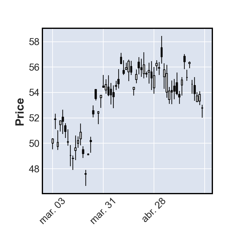
OHLC bars and line
Other values of type are "ohlc" (bars with ticks for the opening and closing prices), "line" and "renko".
import numpy as np
import pandas as pd
import mplfinance as mpf

rng = np.random.default_rng(21)
close = 50 + rng.normal(0, 1, 60).cumsum()
df = pd.DataFrame({"Open": close + rng.normal(0, 0.5, 60),
                   "Close": close,
                   "Volume": rng.integers(1000, 5000, 60)},
                  index = pd.bdate_range("2025-03-03", periods = 60))
df["High"] = df[["Open", "Close"]].max(axis = 1) + rng.uniform(0, 1, 60)
df["Low"] = df[["Open", "Close"]].min(axis = 1) - rng.uniform(0, 1, 60)

mpf.plot(df, type = "ohlc", figsize = (4, 4))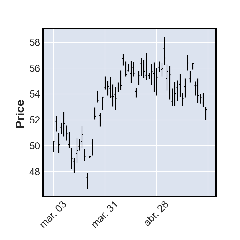
Volume
Set volume = True to add a panel with the traded volume below the candles.
import numpy as np
import pandas as pd
import mplfinance as mpf

rng = np.random.default_rng(21)
close = 50 + rng.normal(0, 1, 60).cumsum()
df = pd.DataFrame({"Open": close + rng.normal(0, 0.5, 60),
                   "Close": close,
                   "Volume": rng.integers(1000, 5000, 60)},
                  index = pd.bdate_range("2025-03-03", periods = 60))
df["High"] = df[["Open", "Close"]].max(axis = 1) + rng.uniform(0, 1, 60)
df["Low"] = df[["Open", "Close"]].min(axis = 1) - rng.uniform(0, 1, 60)

mpf.plot(df, type = "candle", volume = True, figsize = (4, 4))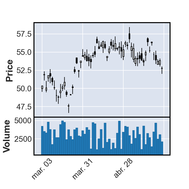
Moving averages
The mav argument adds simple moving averages of the number of periods you specify. Pass a tuple to add several.
import numpy as np
import pandas as pd
import mplfinance as mpf

rng = np.random.default_rng(21)
close = 50 + rng.normal(0, 1, 60).cumsum()
df = pd.DataFrame({"Open": close + rng.normal(0, 0.5, 60),
                   "Close": close,
                   "Volume": rng.integers(1000, 5000, 60)},
                  index = pd.bdate_range("2025-03-03", periods = 60))
df["High"] = df[["Open", "Close"]].max(axis = 1) + rng.uniform(0, 1, 60)
df["Low"] = df[["Open", "Close"]].min(axis = 1) - rng.uniform(0, 1, 60)

mpf.plot(df, type = "candle", mav = (5, 20), volume = True,
         style = "yahoo", figsize = (4, 4))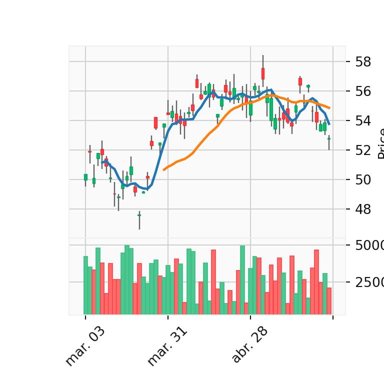
Styles and colors
mplfinance includes several styles, such as "yahoo", "charles", "nightclouds" or "binance" (see them all with mpf.available_styles()). To choose the colors of the candles create a style with make_marketcolors and make_mpf_style.
import numpy as np
import pandas as pd
import mplfinance as mpf

rng = np.random.default_rng(21)
close = 50 + rng.normal(0, 1, 60).cumsum()
df = pd.DataFrame({"Open": close + rng.normal(0, 0.5, 60),
                   "Close": close,
                   "Volume": rng.integers(1000, 5000, 60)},
                  index = pd.bdate_range("2025-03-03", periods = 60))
df["High"] = df[["Open", "Close"]].max(axis = 1) + rng.uniform(0, 1, 60)
df["Low"] = df[["Open", "Close"]].min(axis = 1) - rng.uniform(0, 1, 60)

colors = mpf.make_marketcolors(up = "#2A9D8F", down = "#E76F51", inherit = True)
style = mpf.make_mpf_style(marketcolors = colors, gridstyle = ":")

mpf.plot(df, type = "candle", style = style, figsize = (4, 4))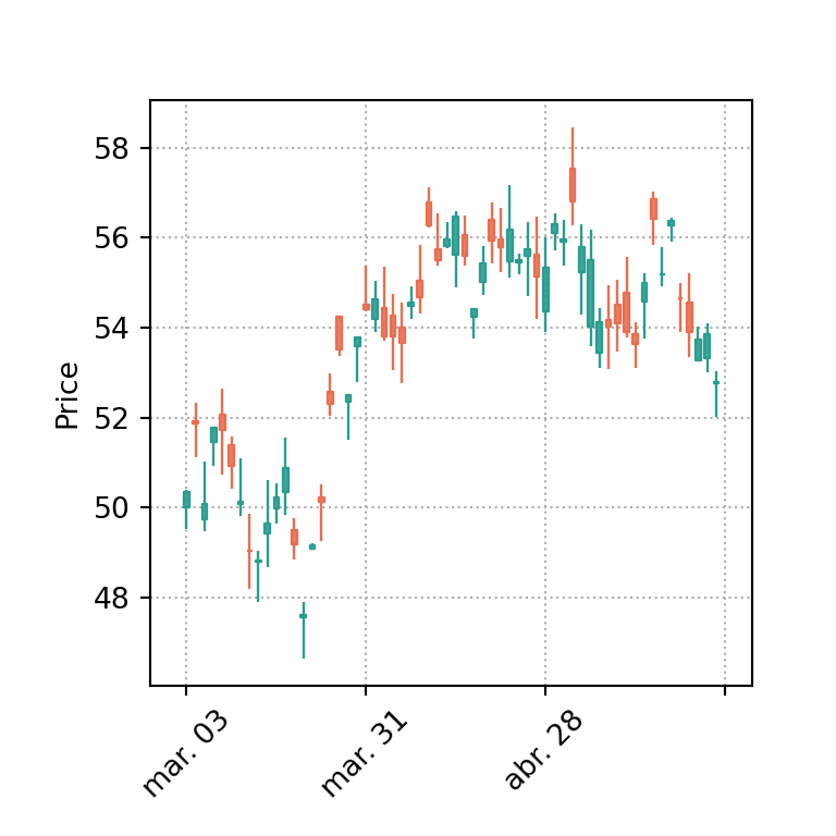
Title and labels
import numpy as np
import pandas as pd
import mplfinance as mpf

rng = np.random.default_rng(21)
close = 50 + rng.normal(0, 1, 60).cumsum()
df = pd.DataFrame({"Open": close + rng.normal(0, 0.5, 60),
                   "Close": close,
                   "Volume": rng.integers(1000, 5000, 60)},
                  index = pd.bdate_range("2025-03-03", periods = 60))
df["High"] = df[["Open", "Close"]].max(axis = 1) + rng.uniform(0, 1, 60)
df["Low"] = df[["Open", "Close"]].min(axis = 1) - rng.uniform(0, 1, 60)

mpf.plot(df, type = "candle", style = "nightclouds", figsize = (4, 4),
         title = "Stock price", ylabel = "Price ($)")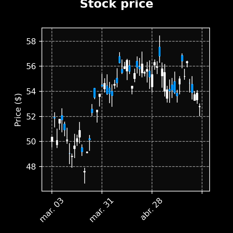
To create an interactive candlestick chart see the candlestick chart in plotly tutorial.