Los ejes de un gráfico de matplotlib están formados por una etiqueta, los límites, los ticks con sus etiquetas y las líneas que rodean el gráfico (spines). Esta guía explica cómo personalizar cada uno de estos elementos.
Etiquetas de los ejes
Agrega una etiqueta a los ejes X e Y con plt.xlabel y plt.ylabel o con los métodos set_xlabel y set_ylabel de los ejes.
import numpy as np
import matplotlib.pyplot as plt

rng = np.random.default_rng(3)
day = np.arange(1, 366)
temp = 15 + 10 * np.sin((day - 110) / 365 * 2 * np.pi) + rng.normal(0, 2, 365)

fig, ax = plt.subplots()
ax.plot(day, temp)

ax.set_xlabel("Día del año")
ax.set_ylabel("Temperatura (ºC)")
# plt.show()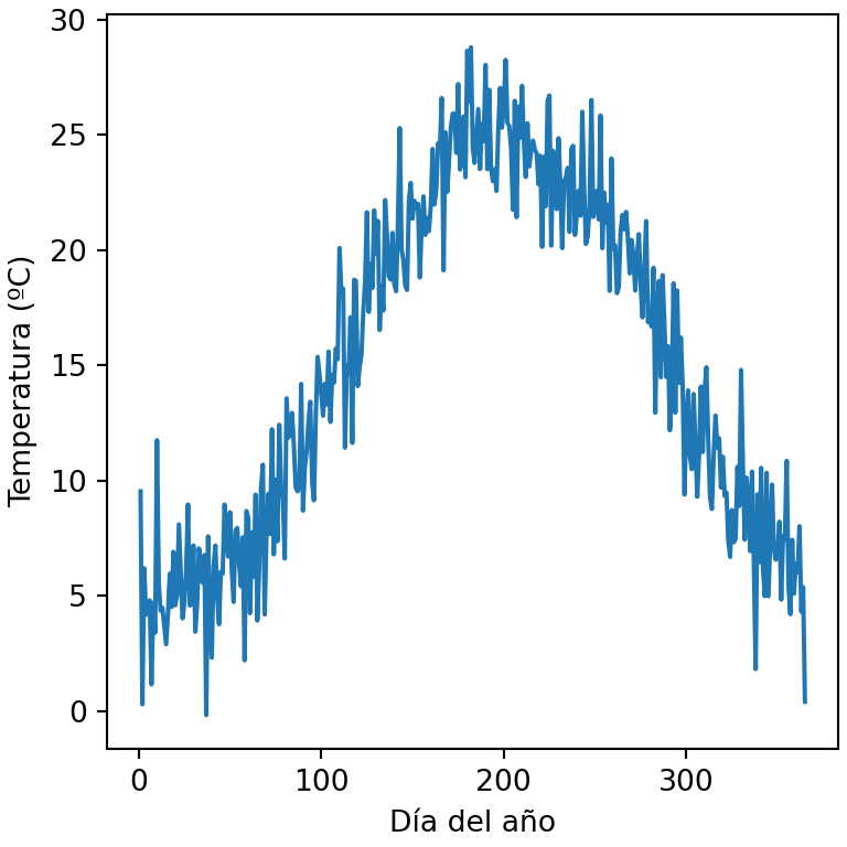
Tamaño, color y distancia de las etiquetas
Los argumentos de texto fontsize, color o fontweight cambian el estilo de las etiquetas, labelpad la distancia al eje y loc su posición ("left", "center" o "right" para el eje X y "bottom", "center" o "top" para el eje Y).
import numpy as np
import matplotlib.pyplot as plt

rng = np.random.default_rng(3)
day = np.arange(1, 366)
temp = 15 + 10 * np.sin((day - 110) / 365 * 2 * np.pi) + rng.normal(0, 2, 365)

fig, ax = plt.subplots()
ax.plot(day, temp)

ax.set_xlabel("Día del año", fontsize = 14, color = "tab:red", loc = "right")
ax.set_ylabel("Temperatura (ºC)", fontweight = "bold", labelpad = 15)
# plt.show()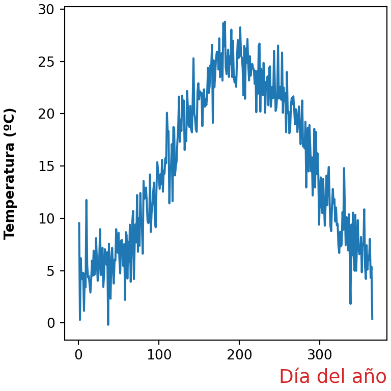
Límites de los ejes
Matplotlib establece los límites automáticamente en función de los datos. Cámbialos con set_xlim y set_ylim (o con plt.xlim y plt.ylim). También puedes establecer solo uno de los límites, como ax.set_ylim(bottom = 0).
import numpy as np
import matplotlib.pyplot as plt

rng = np.random.default_rng(3)
day = np.arange(1, 366)
temp = 15 + 10 * np.sin((day - 110) / 365 * 2 * np.pi) + rng.normal(0, 2, 365)

fig, ax = plt.subplots()
ax.plot(day, temp)

ax.set_xlim(1, 180)
ax.set_ylim(-5, 35)
# plt.show()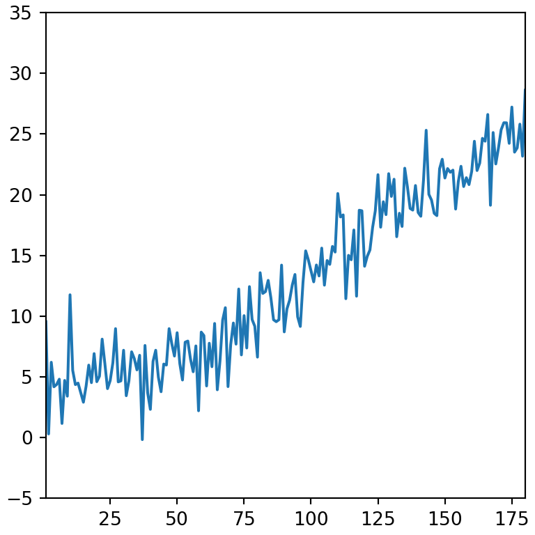
Invertir un eje
Utiliza invert_xaxis o invert_yaxis para invertir la dirección de un eje, o establece los límites en orden descendente.
import numpy as np
import matplotlib.pyplot as plt

rng = np.random.default_rng(3)
day = np.arange(1, 366)
temp = 15 + 10 * np.sin((day - 110) / 365 * 2 * np.pi) + rng.normal(0, 2, 365)

fig, ax = plt.subplots()
ax.plot(day, temp)

ax.invert_yaxis()
# plt.show()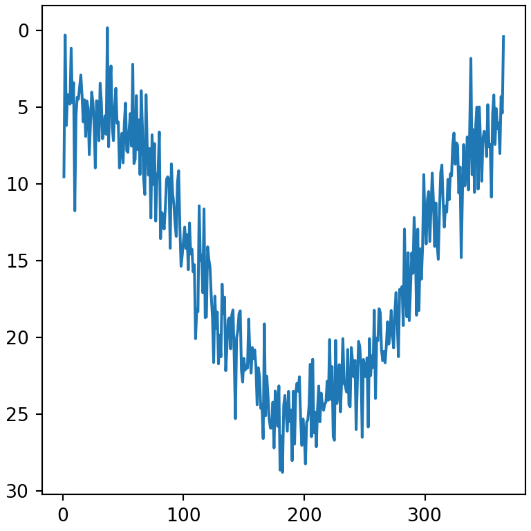
Márgenes
Por defecto hay un pequeño margen entre los datos y los límites. Elimínalo o cámbialo con margins.
import numpy as np
import matplotlib.pyplot as plt

rng = np.random.default_rng(3)
day = np.arange(1, 366)
temp = 15 + 10 * np.sin((day - 110) / 365 * 2 * np.pi) + rng.normal(0, 2, 365)

fig, ax = plt.subplots()
ax.plot(day, temp)

ax.margins(x = 0)
# plt.show()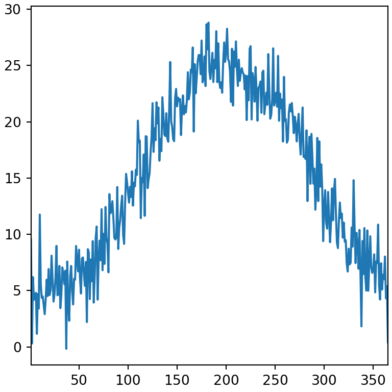
Ticks y etiquetas de los ticks
Establece la posición de los ticks con set_xticks y set_yticks. El argumento labels reemplaza los números por textos personalizados.
import numpy as np
import matplotlib.pyplot as plt

rng = np.random.default_rng(3)
day = np.arange(1, 366)
temp = 15 + 10 * np.sin((day - 110) / 365 * 2 * np.pi) + rng.normal(0, 2, 365)

fig, ax = plt.subplots()
ax.plot(day, temp)

ax.set_xticks([1, 91, 182, 274], labels = ["Ene", "Abr", "Jul", "Oct"])
ax.set_yticks([0, 15, 30])
# plt.show()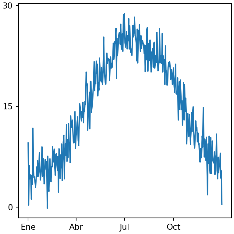
Rotar las etiquetas de los ticks
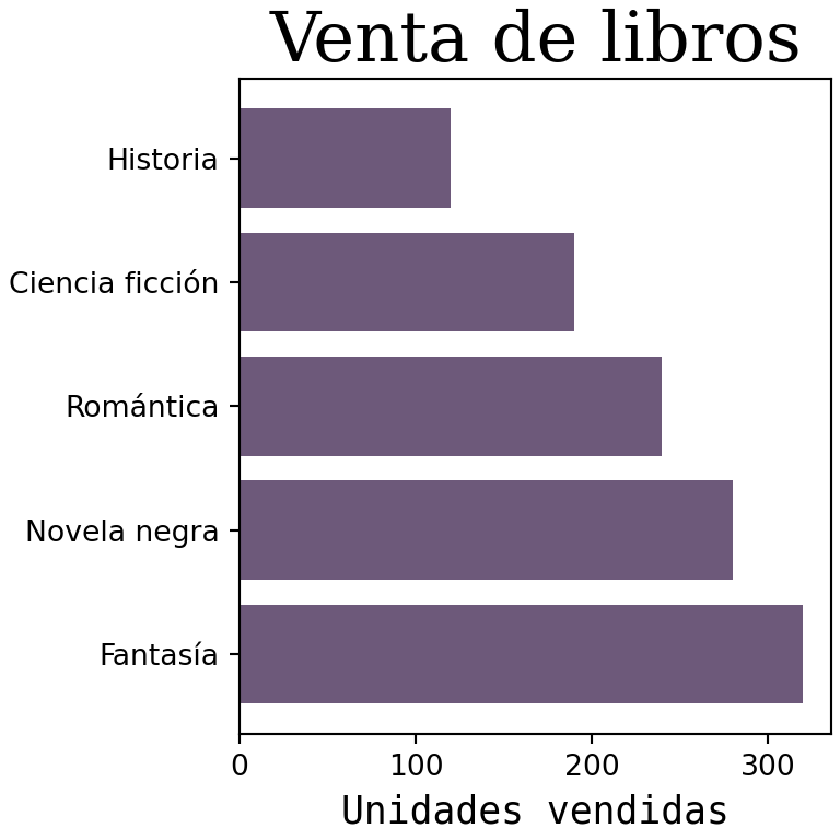
Cuando las etiquetas de los ticks son largas se solapan. Rótalas con el argumento rotation de tick_params o con plt.xticks(rotation = 45).
import matplotlib.pyplot as plt

names = ["Enero", "Febrero", "Marzo", "Abril", "Mayo", "Junio"]

fig, ax = plt.subplots()
ax.bar(names, [5, 7, 3, 8, 6, 9])

ax.tick_params(axis = "x", labelrotation = 45)
# plt.show()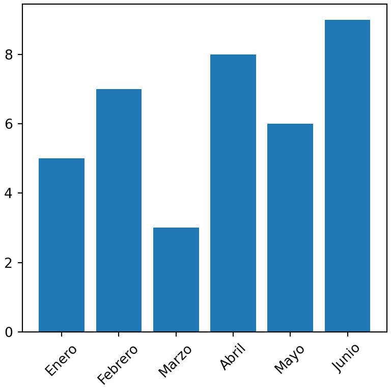
Estilo de los ticks
El método tick_params personaliza los ticks y sus etiquetas: labelsize, labelcolor, length, width, color y direction ("in", "out" o "inout").
import numpy as np
import matplotlib.pyplot as plt

rng = np.random.default_rng(3)
day = np.arange(1, 366)
temp = 15 + 10 * np.sin((day - 110) / 365 * 2 * np.pi) + rng.normal(0, 2, 365)

fig, ax = plt.subplots()
ax.plot(day, temp)

ax.tick_params(axis = "both", labelsize = 12, labelcolor = "tab:blue",
               length = 8, width = 2, direction = "in")
# plt.show()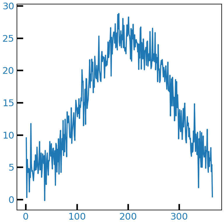
Eliminar los ticks
Pasa una lista vacía a set_xticks o set_yticks para eliminar los ticks y sus etiquetas.
import numpy as np
import matplotlib.pyplot as plt

rng = np.random.default_rng(3)
day = np.arange(1, 366)
temp = 15 + 10 * np.sin((day - 110) / 365 * 2 * np.pi) + rng.normal(0, 2, 365)

fig, ax = plt.subplots()
ax.plot(day, temp)

ax.set_yticks([])
# plt.show()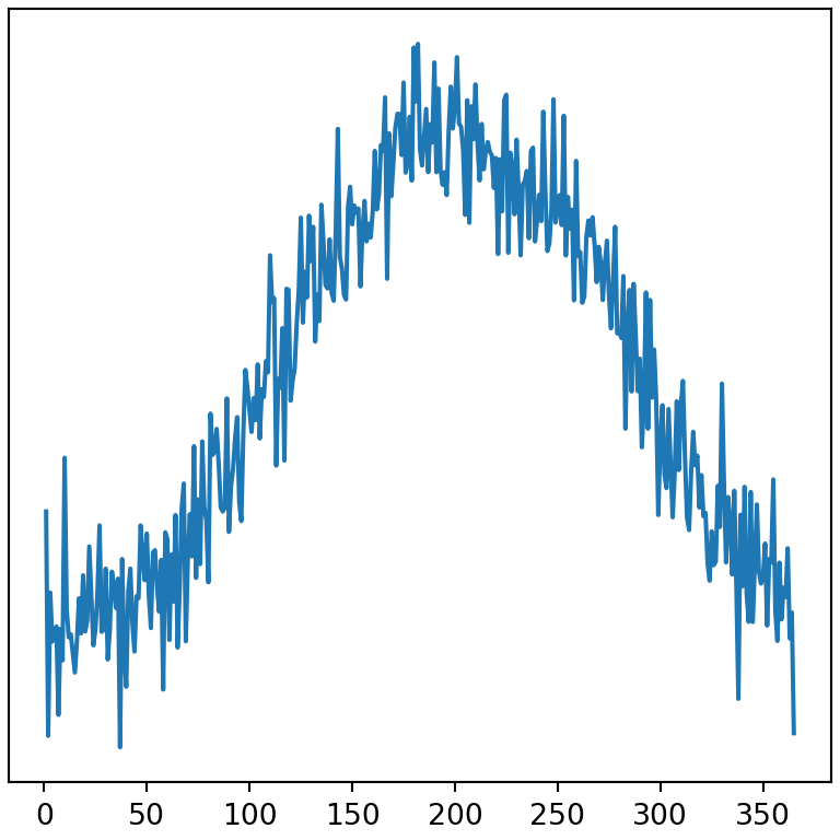
Formato de las etiquetas de los ticks
El módulo matplotlib.ticker proporciona formateadores para mostrar los números de los ejes como porcentajes, como moneda o con separador de miles.
import matplotlib.pyplot as plt
from matplotlib.ticker import PercentFormatter, StrMethodFormatter

fig, ax = plt.subplots()
ax.bar(["A", "B", "C"], [0.25, 0.45, 0.30])

ax.yaxis.set_major_formatter(PercentFormatter(xmax = 1))
# plt.show()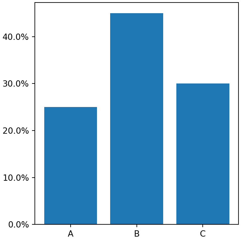
Separador de miles
import matplotlib.pyplot as plt
from matplotlib.ticker import StrMethodFormatter

fig, ax = plt.subplots()
ax.bar(["2023", "2024", "2025"], [125000, 180000, 240000])

ax.yaxis.set_major_formatter(StrMethodFormatter("${x:,.0f}"))
# plt.show()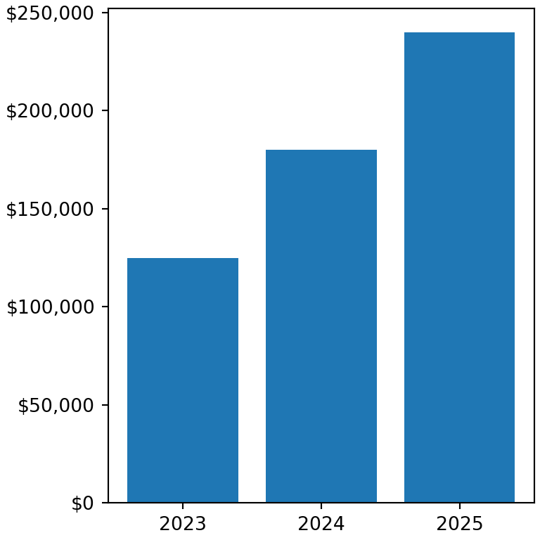
Escala logarítmica
Utiliza set_xscale o set_yscale con "log" para transformar el eje a escala logarítmica. Otras opciones son "symlog" (que admite valores negativos) y "logit".
import numpy as np
import matplotlib.pyplot as plt

years = np.arange(2000, 2026)
devices = 1000 * 1.45 ** (years - 2000)

fig, ax = plt.subplots()
ax.plot(years, devices)

ax.set_yscale("log")
# plt.show()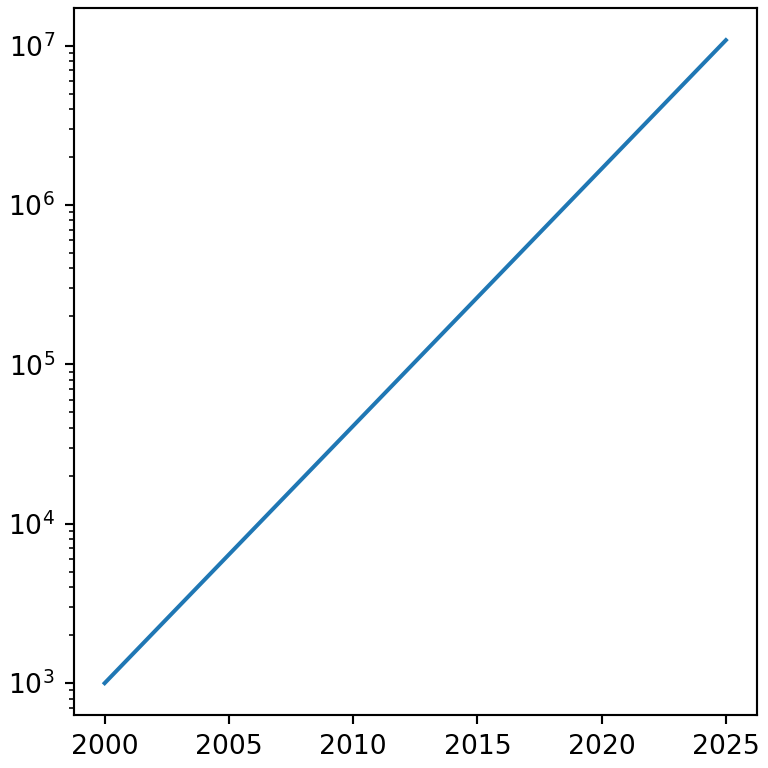
Eliminar los ejes y los bordes
Las líneas que rodean el gráfico se llaman spines. Oculta cualquiera de ellas con set_visible(False) o elimina los ejes completos (bordes, ticks y etiquetas) con ax.axis("off").
import numpy as np
import matplotlib.pyplot as plt

rng = np.random.default_rng(3)
day = np.arange(1, 366)
temp = 15 + 10 * np.sin((day - 110) / 365 * 2 * np.pi) + rng.normal(0, 2, 365)

fig, ax = plt.subplots()
ax.plot(day, temp)

ax.spines[["top", "right"]].set_visible(False)
# plt.show()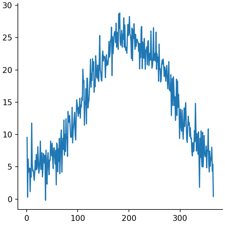
Eje secundario
Para representar dos variables con escalas diferentes en el mismo gráfico crea un segundo eje Y que comparta el eje X con twinx.
import numpy as np
import matplotlib.pyplot as plt

rng = np.random.default_rng(3)
day = np.arange(1, 366)
temp = 15 + 10 * np.sin((day - 110) / 365 * 2 * np.pi) + rng.normal(0, 2, 365)

pressure = 1013 + rng.normal(0, 1, 365).cumsum()

fig, ax = plt.subplots()
ax.plot(day, temp, color = "tab:red")
ax.set_ylabel("Temperatura (ºC)", color = "tab:red")

ax2 = ax.twinx()
ax2.plot(day, pressure, color = "tab:blue")
ax2.set_ylabel("Presión (hPa)", color = "tab:blue")
# plt.show()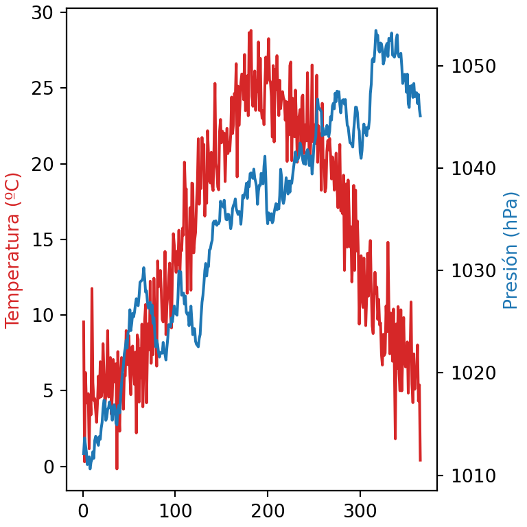
Aprende también a agregar líneas de grid, títulos y textos a tus gráficos de matplotlib.