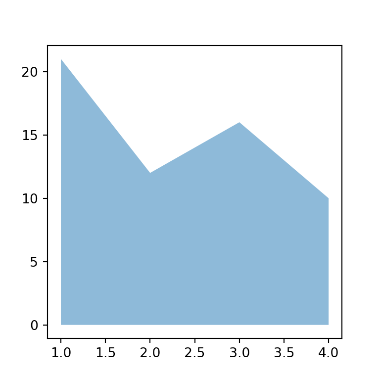
Un streamgraph es un gráfico de áreas apiladas cuyas áreas se colocan alrededor de un eje central en lugar de sobre el cero, lo que le da un aspecto orgánico y fluido. Es útil para mostrar cómo cambia la composición de un total a lo largo del tiempo. Los ejemplos muestran la evolución de la cuota de escucha de varios géneros musicales.
Streamgraph con stackplot
stackplot apila las series. Establece baseline = "wiggle" para centrarlas y minimizar la pendiente de las capas, lo que crea el streamgraph.
import numpy as np
import matplotlib.pyplot as plt

years = np.arange(2000, 2026)
t = (years - 2000) / 25
genres = ["Pop", "Rock", "Hip hop", "Electrónica", "Latin"]
listens = np.vstack([30 + 5 * np.sin(6 * t),
                     35 - 25 * t,
                     5 + 30 * t,
                     8 + 12 * np.sin(3 * t) ** 2,
                     3 + 25 * t ** 2])

fig, ax = plt.subplots()
ax.stackplot(years, listens, labels = genres, baseline = "wiggle")
ax.legend(loc = "upper left", fontsize = 8)
# plt.show()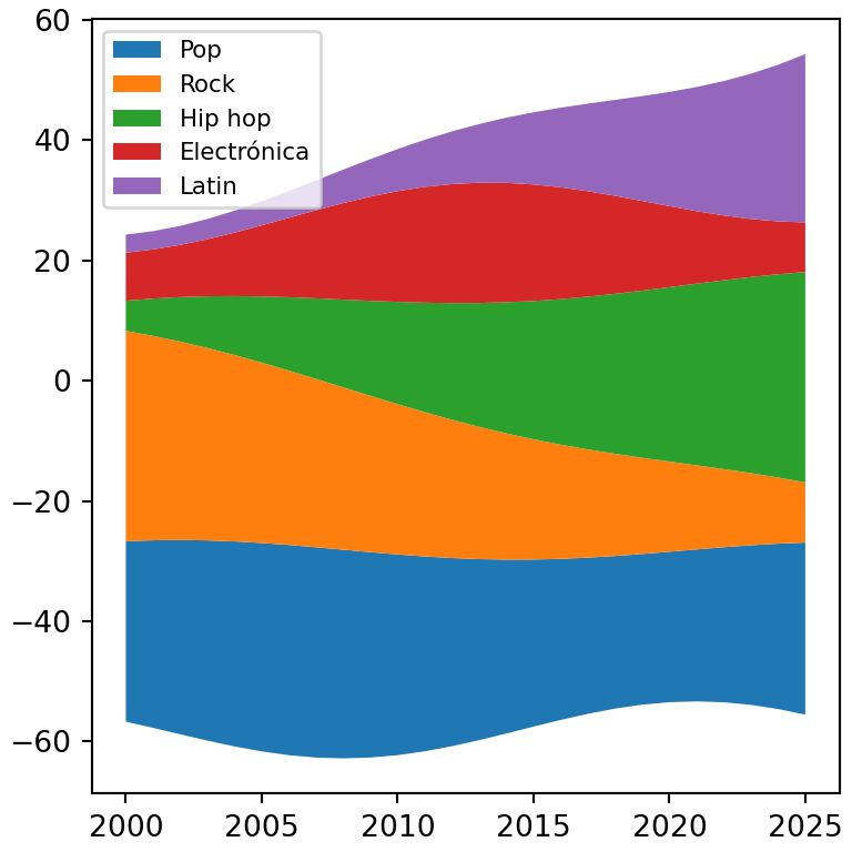
Líneas base
Otras opciones de baseline son "zero" (un gráfico de áreas apiladas normal), "sym" (simétrico alrededor del cero) y "weighted_wiggle".
import numpy as np
import matplotlib.pyplot as plt

years = np.arange(2000, 2026)
t = (years - 2000) / 25
genres = ["Pop", "Rock", "Hip hop", "Electrónica", "Latin"]
listens = np.vstack([30 + 5 * np.sin(6 * t),
                     35 - 25 * t,
                     5 + 30 * t,
                     8 + 12 * np.sin(3 * t) ** 2,
                     3 + 25 * t ** 2])

fig, ax = plt.subplots()
ax.stackplot(years, listens, baseline = "sym")
# plt.show()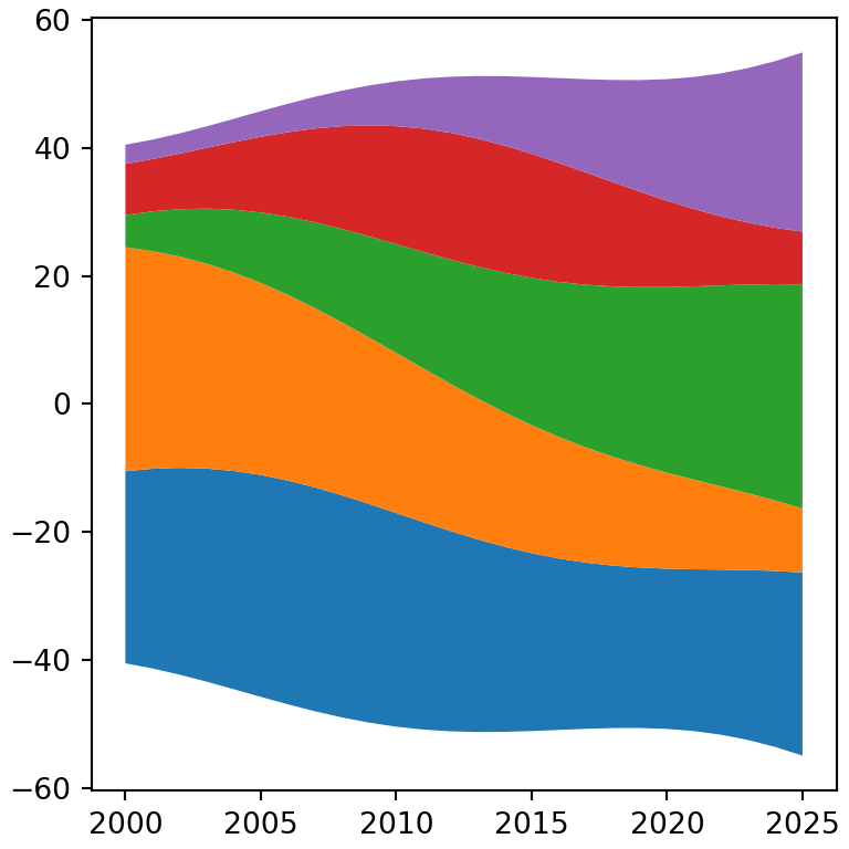
Corrientes suavizadas
Con pocos puntos las corrientes se ven angulosas. Interpola los datos con un spline de scipy para obtener curvas suaves.
import numpy as np
import matplotlib.pyplot as plt

years = np.arange(2000, 2026)
t = (years - 2000) / 25
genres = ["Pop", "Rock", "Hip hop", "Electrónica", "Latin"]
listens = np.vstack([30 + 5 * np.sin(6 * t),
                     35 - 25 * t,
                     5 + 30 * t,
                     8 + 12 * np.sin(3 * t) ** 2,
                     3 + 25 * t ** 2])
from scipy.interpolate import make_interp_spline

x_smooth = np.linspace(years.min(), years.max(), 300)
y_smooth = make_interp_spline(years, listens, k = 3, axis = 1)(x_smooth)

fig, ax = plt.subplots()
ax.stackplot(x_smooth, y_smooth, baseline = "wiggle",
             colors = ["#264653", "#2A9D8F", "#E9C46A", "#F4A261", "#E76F51"])
ax.axis("off")
# plt.show()
Etiquetas sobre las corrientes
En lugar de una leyenda puedes escribir el nombre de cada grupo sobre su corriente. Calcula dónde está cada capa en un valor de X concreto y coloca ahí el texto.
import numpy as np
import matplotlib.pyplot as plt

years = np.arange(2000, 2026)
t = (years - 2000) / 25
genres = ["Pop", "Rock", "Hip hop", "Electrónica", "Latin"]
listens = np.vstack([30 + 5 * np.sin(6 * t),
                     35 - 25 * t,
                     5 + 30 * t,
                     8 + 12 * np.sin(3 * t) ** 2,
                     3 + 25 * t ** 2])

fig, ax = plt.subplots()
ax.stackplot(years, listens, baseline = "wiggle", colors = plt.cm.Set2.colors)

i = 18
bottom = -listens[:, i].sum() / 2
for name, value in zip(genres, listens[:, i]):
    ax.text(years[i], bottom + value / 2, name, ha = "center", va = "center")
    bottom += value
ax.set_yticks([])
# plt.show()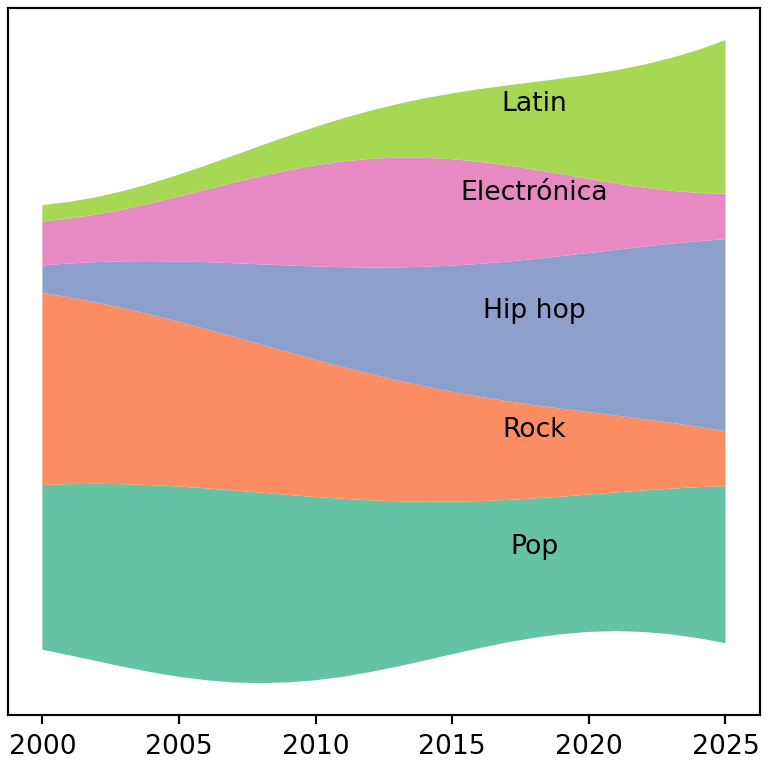
Consulta también cómo crear un gráfico de áreas apiladas en matplotlib.